
Part II · Chapter 09
Creating Custom & Uploaded Components
When the catalog does not have the part you need, build one from your own specification.
The custom optics form
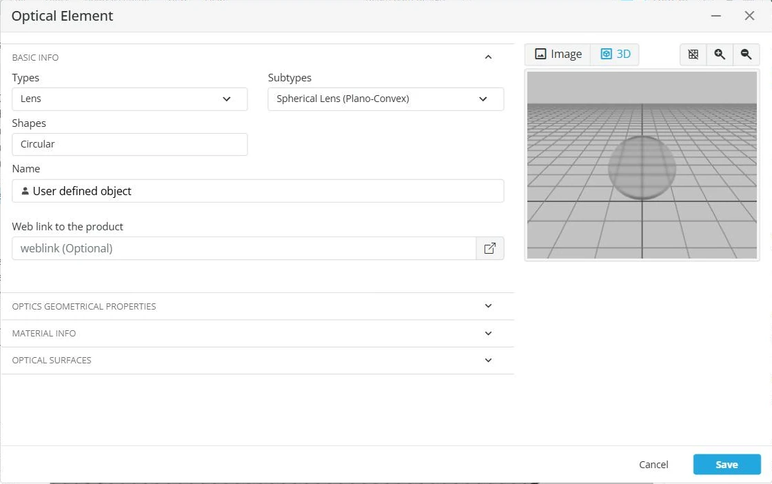
Open the form by dragging Create custom <Type> from a catalog results page, or the Custom Lens Quick Add chip, onto the canvas. One form serves every optics type; its sections change with the type:
| Section | What it holds |
|---|---|
| Basic Info | Type, subtype, shape, name and an optional product link. |
| Physical Info | Physical parameters of the part. |
| Geometrical Info | Shape and dimensions. |
| Material | One entry per element; a doublet or triplet has several. |
| Surfaces | The list of faces. Select one to edit it. |
| Deformation Settings | Per face: flat, conic or asphere. |
| Face Simulation Settings | Per face: non-reflecting (the default) or reflecting with a Max bounces limit of 0 to 50. |
| Coating | Upload polarization-dependent transmission and reflection data. |
| Scattering | Stray-light behavior. |
| Parametric Aperture | An adjustable inner and outer aperture. |
| User Aperture (Mask) | Upload a transmission mask image. |
| Polarizer Info | For the Polarizing Element type. |
| Ideal Objective, Objective Lens Tube | For the Ideal Microscope Objective type. |
| Ideal Beam Expander | For the Ideal Beam Expander type. |
Changing a material is Professional-tier.
Faces
A custom optic is built from faces. Select a face in the Surfaces list, then set its deformation, simulation settings, coating and scattering. Each face has its own settings.
Coating data
The Coating section takes a .csv or .xlsx file with transmission and reflection per wavelength for P and S polarization, optionally with phase. Download Template gives you the column layout.
Which face carries the coating: on a cube beam splitter, including the polarizing cube, it is the diagonal face; on a thin beam splitter, the front face.
The values are power, not amplitude. Enter Rs, Rp, Ts and Tp as fractions of power. A reflectance of 0.8 means 80% of the incident S-polarized power is reflected.
Angle of incidence. The file's values are applied as they are, at every angle. The tool still works out the S and P directions for each ray from its own angle and the surface at the hit point.
Polarization
3DOptix traces polarization in 3D for every ray at every surface. At each hit it finds the plane of incidence for that ray, splits the ray's polarization into local S and P components, and applies the Fresnel coefficients for the wavelength, the materials and the angle. This holds for folded paths such as a two-mirror periscope, for tilted surfaces and for strongly curved ones. The X, Y and Z components shown in analysis results are the resulting state expressed in the analysis coordinate system.
- Ideal polarizer and polarizing beam splitter apply a set Jones matrix.
- Ideal wave plate models birefringence: you enter the ordinary and extraordinary indices, and the tool traces separate ordinary and extraordinary rays, each refracted with its own index.
- Uncoated surfaces use Fresnel coefficients from the ray's angle and the two refractive indices, including total internal reflection.
- Not modeled: birefringence from a crystal material such as calcite or quartz assigned to an ordinary lens or window. Use the Ideal Wave Plate for that.
Scattering
The Scattering section sets stray-light behavior for a face. For every model you set:
- Transmittance / Reflectance / Absorption, as percentages.
- Relative power threshold, below which scattered rays are dropped.
- Scattering percentage, the share of the light that is scattered rather than reflected or transmitted directly.
- Number of scattered rays per hit.
Each model gives the scattered intensity I as a function of the angle θ from the model's axis, and for the Gaussian model also of the azimuth φ. I0 is the intensity on the axis. Gaussian, Super Gaussian and ABg are centered on the direction of specular reflection or refraction; Lambertian and Cos-Nth on the surface normal.
| Model | Distribution | Parameters |
|---|---|---|
| Gaussian | I(θ, φ) = I0 · exp(−(θ²/2) · (cos²φ / σx² + sin²φ / σy²)) | σx, σy: the width of the lobe along the local x and y axes. |
| Super Gaussian | A Gaussian with an extra order parameter that flattens the peak. | σx, σy and the order. |
| Lambertian | I(θ) = I0 · cos θ | None. A matte surface. |
| Cos-Nth | I(θ) = I0 · cosN θ | N: 1 is Lambertian; larger values narrow the lobe. |
| ABg | I(θ) = A / (B + |β − β0|g), where β = sin θ and β0 = sin of the specular angle | A, B, g: A/B sets the peak, B the width of the flat top, g the fall-off of the wings. |
Parametric aperture
The Parametric Aperture section builds an aperture from an inner opening and an outer frame. Each is Elliptical (radius X, radius Y) or Rectangular (half width, half height), set with sliders in your working units.
Masks
The User Aperture (Mask) section takes a .png image and uses its transparency as the aperture shape.
Ideal objective and beam expander
Ideal Microscope Objective and Ideal Beam Expander are defined by their first-order behavior, such as magnification or expansion ratio, with no lens prescription behind them. Use them to lay out a system before choosing real parts.
Light source settings
Select a light source to see its settings in the Inspector, below Move & Rotate.
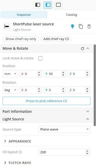
Source type
Point source, Plane wave, Omnidirectional point source (when enabled for your account) and Gaussian (Professional-tier). A user-defined light source can also be a Screen source, a Custom beam source or an LED, depending on your account.
Spatial and angular settings
For plane waves and point sources, Spatial information sets the shape (circular, elliptical, square or rectangular), the size and the ray pattern (random, periodic, circular or grid). Angular information sets the direction, as angles in degrees or mrad or as direction cosines, plus the azimuth for non-circular shapes. A point source also has a divergence: a half-cone angle, a half-width angle or a half width at a given distance.
Wavelengths
Spectrum type offers four models:
| Spectrum type | Parameters |
|---|---|
| User-defined | Add wavelengths and their weights by hand. |
| TH | λmin, λmax and the step. |
| Gaussian | Central wavelength and width. |
| Blackbody | Temperature. |
For the last three, Apply generates the wavelength list. One wavelength is marked primary; it is used for calculations and cannot be deleted. You can move the primary mark to another wavelength.
Polarization
Every source starts unpolarized. Type of polarization offers several equivalent ways to set a state:
- Orientation angle (−180° to +180°) and Eccentricity (0 for circular to 1 for linear).
- Ellipticity angle and Extinction ratio (0 to 100).
- Polarization angle: one angle, from which the Jones vector is computed.
- Jones vector: principal and orthogonal Jx and Jy, real and imaginary parts.
- Stokes parameters: S0, S1, S2, S3.
- Phase shift and auxiliary angle.
- Circular Left or Circular Right.
Editing any field marks the source User Defined. To return to unpolarized light, choose the unpolarized option in Type of polarization rather than clearing the fields.
Number of rays
A source has two ray counts. 3D Layout is the number of rays drawn in the viewport, 30 by default and up to 200 in Fast Rays mode; it affects only the display. The Analysis count, 1,000,000 by default, is traced by a Propagation Simulation, and each analysis can override it in the Analysis Portal. Raise the layout count when a tool measures the drawn rays, such as the Gaussian Beam tool.
Power
The source power, in watts.
Uploading a measured light source
The Ray File tile in the Light Sources category imports a source profile in the IES-TM25 format. It is not enabled on every account.


