Home

Temporal Coherence

Temporal Coherence

In optics, coherence is a function of the wave nature of light which describes phase as it travels through a medium. In classical geometric optics, light is often described as rays and is particularly  effective when dealing with situations where the wavelength of light is much smaller than the size  of objects and apertures involved, and wave effects such as interference and diffraction are negligible. Temporal Coherence is crucial for interference phenomena, such as Young’s double-slit  experiment. When light waves are temporally coherent, they can produce a stable interference  pattern. Lasers, long temporal coherence, and LED’s, short temporal coherence, are used in many  optical applications where interference effects are required.

The coherence length of a source can be described by L_C=\frac{\lambda}{\Delta \lambda}, where \lambda is the center wavelength of the source and \Delta \lambda is the spectral bandwidth.

Using either manufacturer data or knowing the source specifications we wish to simulate we can estimate the coherence length and build optical systems to observe interference effects.

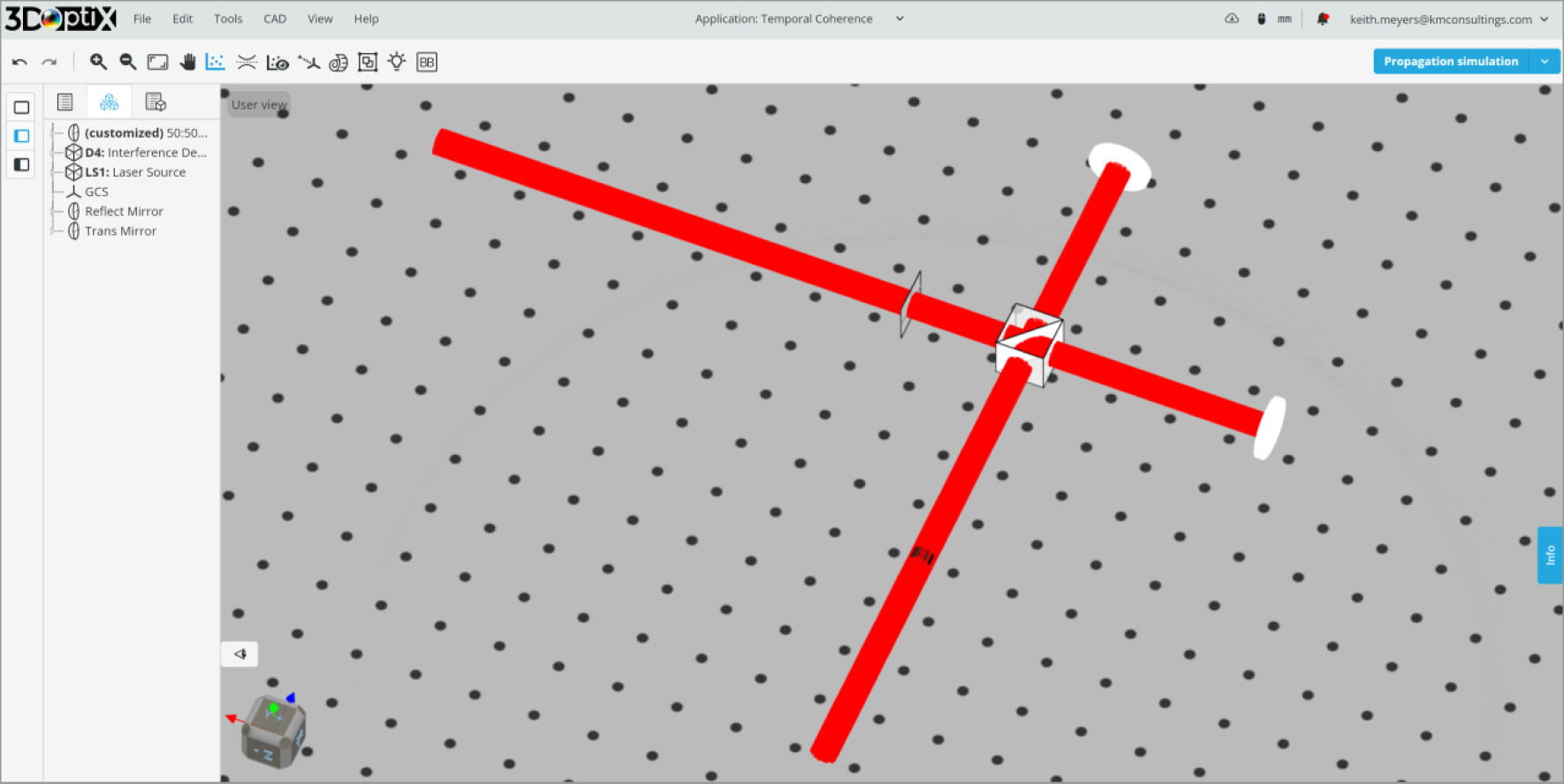
In 3DOptix cloud-based simulation tool these systems can easily be designed and tested using the light sources, optics, and analysis features available. We will overview one application with use cases to get more familiar with these designs.

Our optical system will consist of a Michelson interferometer with the following components:
  • Perfect Dielectric 1” Mirror
  • Perfect Dielectric 1” Mirror
  • Perfect 1” Cube Beamsplitter 50:50 (R:T) Uncoated
  • Light Source
    1. Plane Wave
    2. Rectangular, 5×5 mm half dimensions
    3. 633 nm wavelength
    4. Power, 1 W
    5. Unpolarized
  • Detector: Illumination
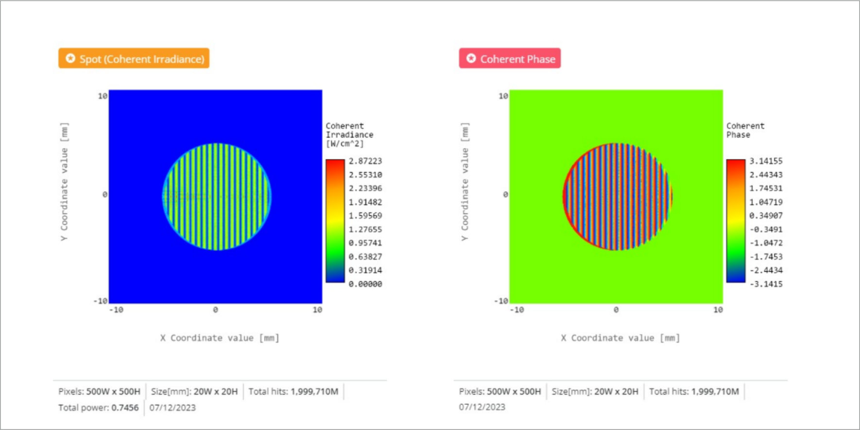
    1. Spot: Coherent Irradiance
    2. Analysis Rays: 1 million
    3. 500×500 pixels
You can see the image of our optical system below. The 3DOptix simulation file can be downloaded to see additional information about the optical system such as component spacing and analysis detectors. Note that the perfect beamsplitter has a 50:50 coating automatically applied, but we have the ability to change this coating.
Using the CUSTOM FILE button an excel file will be downloaded. In the spreadsheet the second row defines a wavelength, wl, with the transmission, t_p and t_s, and reflection, r_p and r_p properties for each polarization state. These values can be changed as long as the sum of the transmission and reflection each equal 100%.
Using a Michelson interferometer, we can observe the temporal coherence of the optical system. The two mirrors will be placed at the same distance from the beamsplitter to generate a baseline  measurement with maximal fringe contrast. We need to tilt one of the mirrors or the beamsplitter so that we are able to observe fringes as the wavefront is flat due to the perfect optics we are  using in this system. We will choose to rotate the reflected path mirror by 0.05 degrees. 
If we move the reflected path mirror farther away, we will change the interference pattern, but since we are simulating a laser, we will only see a shift in the fringe pattern that will eventually  repeat.
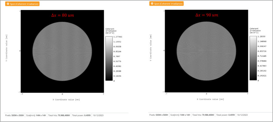
This is the idea behind Fourier Transform Infrared (FTIR) spectrometers that measure the  spectrum of a light source. Moving the reference mirror through a certain distance will allow one to measure the spectrum using the interference fringes, and once you have moved the mirror  through one full cycle the pattern repeats. By altering the reflected path mirror we can experimentally confirm that the coherence length we calculate is accurate.
Next, instead of using an ideal laser at a single wavelength we will now model a real laser with a finite spectral bandwidth which will generate a shorter temporal coherence length. The parameter we need to change to achieve this is the spectrum of the light source. Previously, we only specified a single wavelength to simulate the ideal laser, but now we will add many more to shorten the coherence length as per the coherence length L_C=\frac{\lambda}{\Delta \lambda}

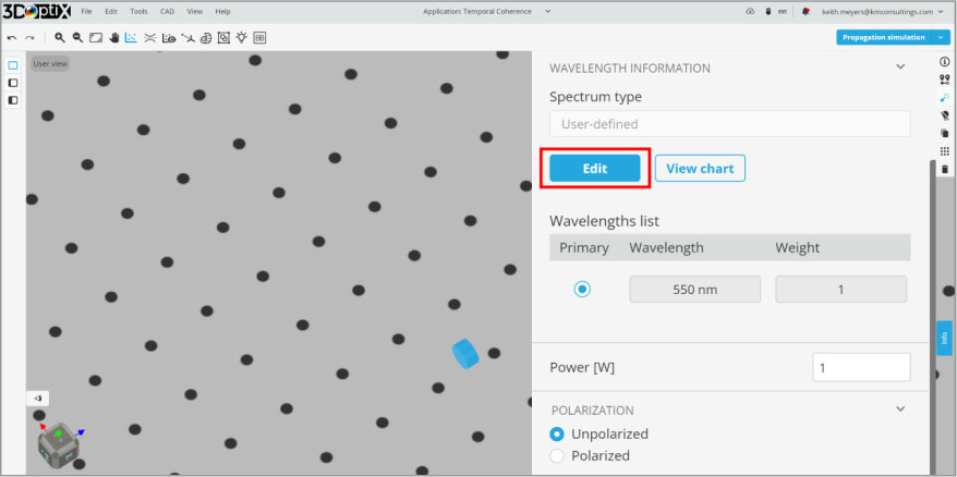
An additional parameter we want to use for the plane wave light source is the SPECTRUM TYPE. By including additional wavelengths to simulate an LED we can change the coherence length previously described.

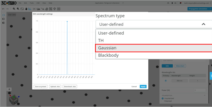
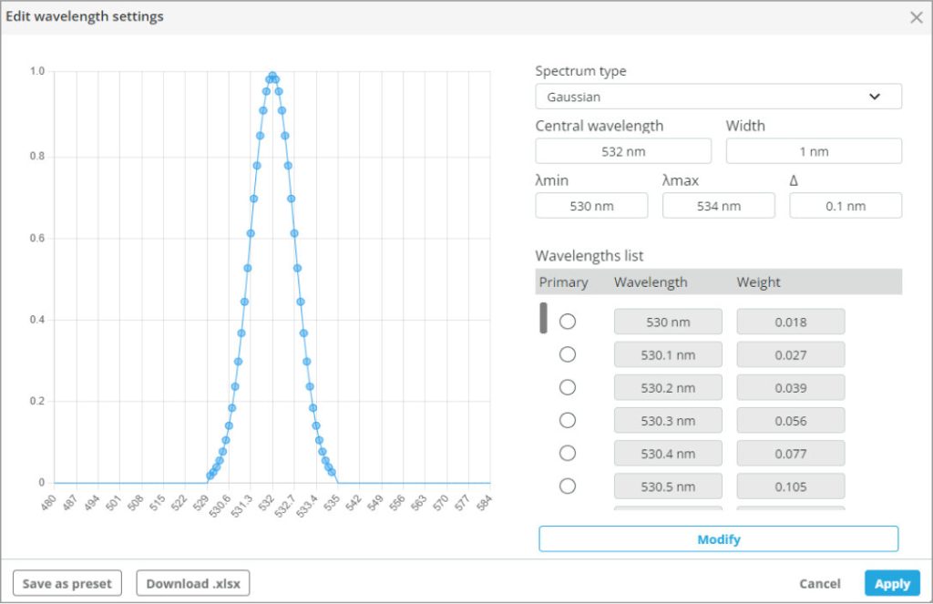
For this system, we will add a GAUSSIAN spectral distribution around the central wavelength of 532 nm. This will change our coherence length from infinite, due to the single wavelength, to some finite length.

One quick note, you can change the colormap range to better see the image of the interference fringes.
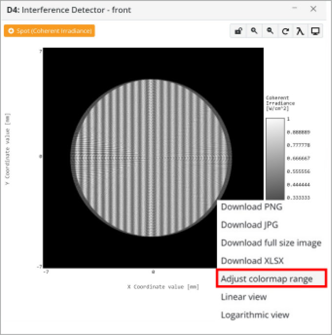
If we click on the analysis image it will pop out into its own window and on the bottom right, we can click on the three bars icon. This will bring up the options drop-down.
Now we can re-analyze the system to determine the interference pattern from the real laser and its corresponding coherence length.
The mirror on the reflected side of the beam splitter is shifted 10 um from the beam splitter until fringes are no longer visible. The path length will be twice the deviation by the mirror shift. Note that the total power and total hits do not change since we are only observing different fringes patterns, not changing the energy on the detector.
We can see that the fringe contract becomes very poor on the detector at a mirror shift of 80 um, and then indistinguishable at a mirror shift of 90 um.
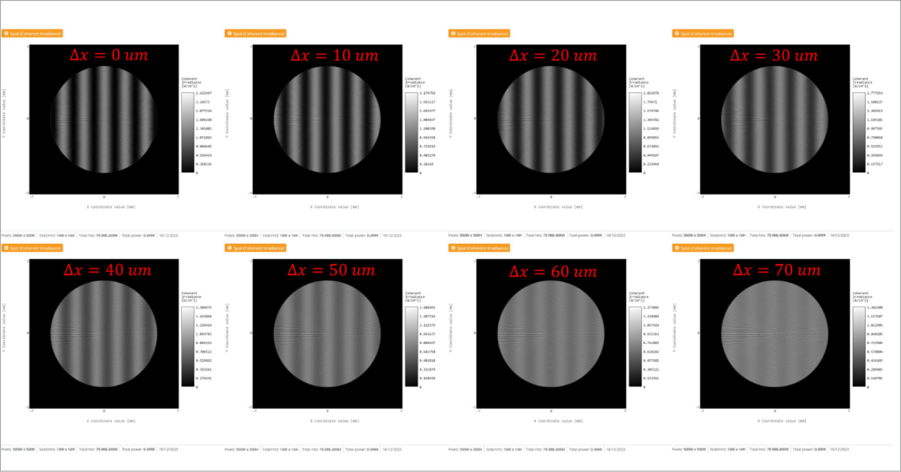
We can calculate the coherence length of the simulated light source based on our user generated spectral width of 1.7 nm FWHM.
The coherence length in our simulated light source is thenLC = 166 um. We have achieved observable fringes for a total path length of 160 um, which agrees well with theory.
mascot-1-1

3DOptix works
only on desktop!

Please go to 3doptix.com on a
desktop device, using the
Chrome or Edge browser

Available on January 30th, 2023