- 2x Light Sources
- Plane Wave
- Circular, 4 mm radius
- 800 nm wavelength
- Power, 1 W
- Linearly Polarized, 0 degrees
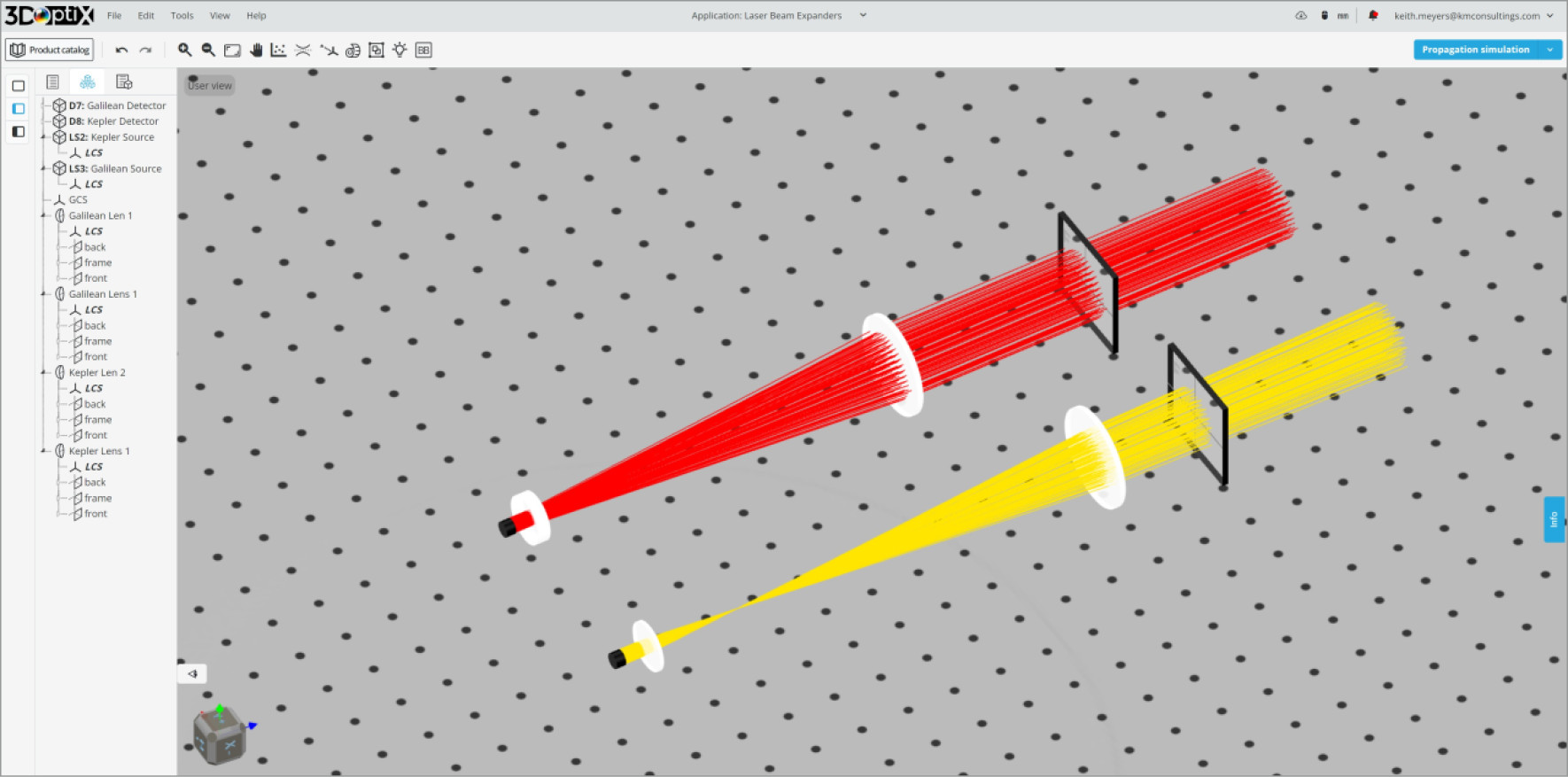
- Kepler Beam Expander
- Thorlabs LA1131, 50 mm FL Plano-Convex
- Thorlabs LA1301, 250 mm FL Plano-Convex
- Galilean Beam Expander
- Thorlabs LC1259, -50 mm FL Plano-Concave
- Thorlabs LA1301, 250 mm FL Plano-Convex
- 2x Detectors
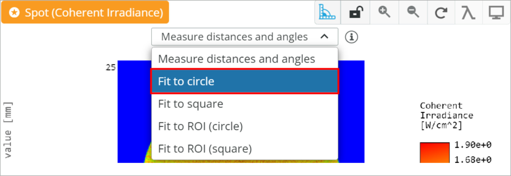
- Spot: Coherent Irradiance
- Analysis Rays: 1 million
- 300×300 pixels
- Lens Separation: D = f_{lens1} + f_{lens2}
- System Magnification: M = \frac{f_{lens2}}{f_{lens1}}
- D_{Kepler} = 50 mm + 250mm = 300mm
- M_{Kepler} = \frac{250mm}{50mm} = 5x
- D_{Galilean} = -50 mm + 250mm = 200mm
- M_{Galilean} = \frac{250mm}{-50mm} = 5x
Now, we must place the lenses in the correct location so that a collimated input light is still collimated at the output. We shall go to the lens properties and use the design wavelength we specified to find the back focal length (BFL) of the lenses.
The lenses’ Plano sides will face each other to reduce aberrations. This is a common technique as the Plano side has no optical power when collimated light is incident normal to the surface. By making the rays refract and exit the Plano side at an angle we can “split” the aberrations between each surface reducing them overall.
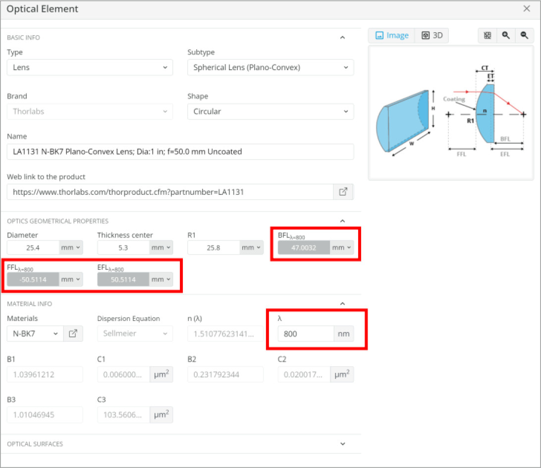
- D_{Kepler} = 47.0032 mm + 248.5247 mm = 295.5279 mm
- D_{Galilean} = -52.6323 mm + 248.5247 mm = 195.8924 mm
These changes are not significant and easily understood and calculated. Therefore, as the system is built this method is preferential.
To simplify the positioning of the lenses, we will perform additional steps. When setting the object position in the 3D layout, the surface with the local coordinate system (LCS) attached to it is positioned at the specified location. That is, if a lens is placed at z=150 mm, then the surface that has the LCS is placed at that point.
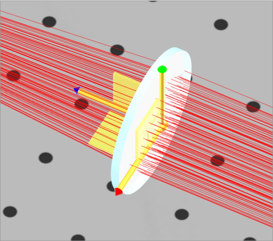
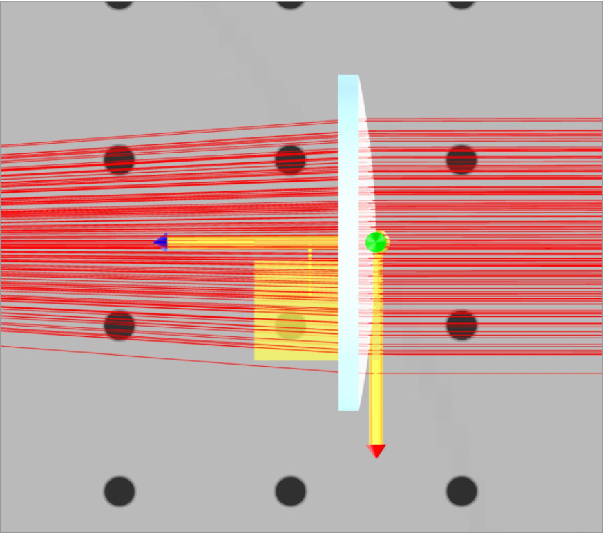
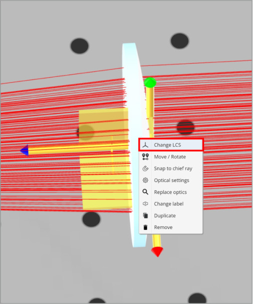
We will change the LCS for lens 2 in both beam expander systems. For the plano-convex lens, the LCS is attached to the front, or curved, surface. This is displayed when you click on the lens. Note that the blue-axis indicator always goes through the opposite surface to which it is referenced. This is an easy way to tell which surface has the LCS at a glance.
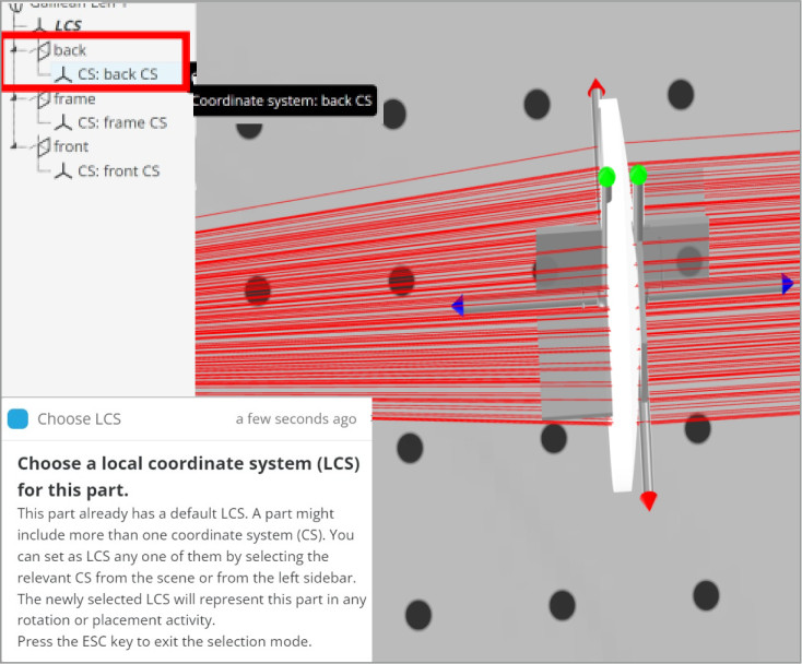
We want the Plano side of the Plano-convex lens to be the LCS so that the separation between the two lenses can be calculated directly from the Plano side to the Plano side. Otherwise, we would need to subtract the thickness of the plano-convex lens from the separation to get the correct position. We will reference lens 2, plano-convex, of both Kepler and Galilean beam expanders to the back of lens 1, plano-convex, and plano-concave lenses respectively.
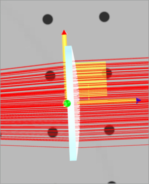
Note that when we click on the plano-convex lens the blue axis indicator now points the other way.
With the lenses for both beam expanders positioned correctly, we will analyze the magnification. We are expecting that the 8 mm diameter input beams, the initial specification, will increase by 5x to 40 mm in diameter. We will use the measuring tool in the analysis window to get a good estimate of the beam diameters.
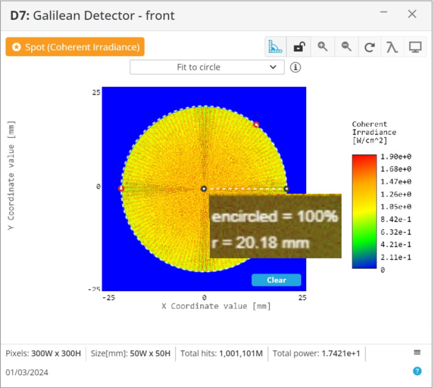
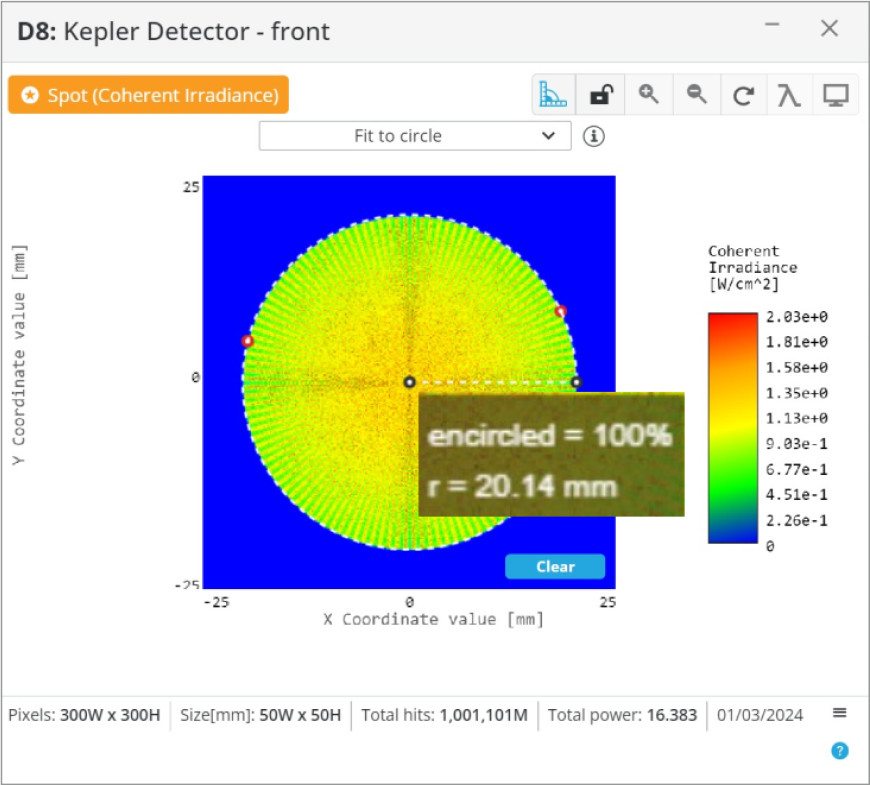
From the analysis of the output beams, it appears that the magnification is correct at ~5x. We can now implement this in a larger optical system, or further optimize the systems to our specific application.
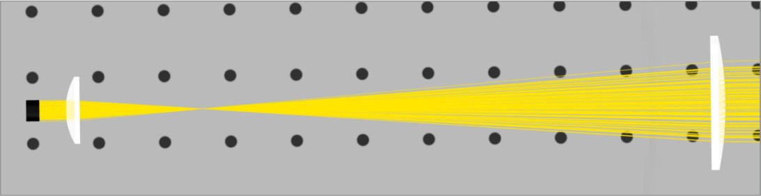
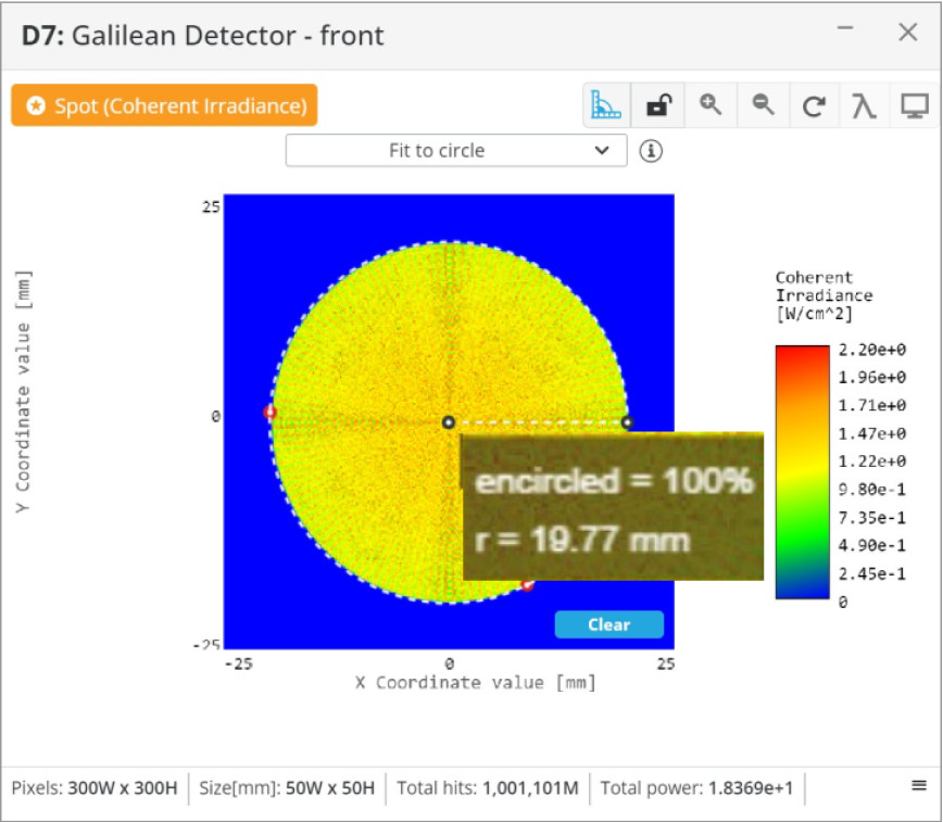
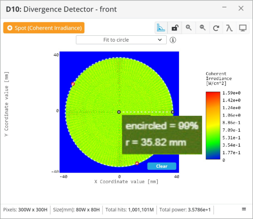
To show the versatility of the beam expander we will take the Galilean beam expander and move lens 2 slightly to give the output beam some divergence. Conversely, we could move lens 2 to the right to create a converging beam. This is a useful application if we need to couple the laser beam into another optical system that has a certain acceptance angle, or if we need a certain spot size at a specific distance. We will move lens 2 to the left 10 mm, then place two detectors 1000 mm apart to measure the divergence.
Some characteristics are common to beam expander systems and others are unique to the ones we have reviewed.
- Reduced power density as the beam diameter is magnified, so damage to sensitive optical surfaces can be eliminated. This is given as the laser-induced damage threshold (LiDT) of optics specified in W/cm^2 or J/cm^2.
- Larger input beam diameters can be focused on a smaller spot size.
- Can also be reversed to demagnify an input beam. This can be useful if the LiDT of a set of optics in an optical system has a lower value than others and the power density needs to be reduced by expanding the beam, then expanded later on in the system.
- The input and output beam can be collimated, diverging, converging, or a combination of these giving versatility to the system for multiple applications.
- Longer total system lengths as focal lengths are added to get lens separation.
- Internal focus can be impossible to use with high power pulses laser due to ionization of the air at the focus.
- Shorter total system length as focal lengths are added to get lens separation.
- No internal focus making it a better option for high-power pulsed lasers.
- Reduced aberrations as the negative and positive lenses used cancel them to an extent


