Introduction
Light is more than just beams traveling from sources, it is an electromagnetic wave. Usually, we do not feel the wave property of light and can analyze the system as beams traveling in straight lines. The understanding that light is more than just beams was revealed by the combined work of Poisson, Fresnel, and Maxwell during the 19th century. Maxwell developed a set of equations that describe the connection between the electric and magnetic fields and how light waves propagate in space. One of the most important properties of waves is the ability to interfere with other waves leading to constructive interference when two waves are in phase, so they are enhancing each other, or destructive interference when the two waves are out of phase resulting in a weaker signal than the waves on their own.
The waves are similar to waves in the ocean, they have frequency and wavelength. The frequency describes how rapidly each point is moving up and down. High frequency means that there is a short time between each cycle and low frequency means that there is a long time between each cycle. The wavelength of a wave describes how far two adjacent peaks are. Long wavelength means that the peaks are separated far from each other, and short wavelength means that the peaks are closer. The relation between and the frequency of the wave and its wavevector is called the dispersion curve and it depends on the optical property of the material.
A periodic series of sources generates a beam at a specific angle where all the sources constructively interfere with each other. This happens when the distance differences between each adjacent source are an integer number of the wavelength. This is illustrated in Fig. 1(a) and leads to the Bragg equation
\sin(\theta_n)=\frac{n\lambda}\Lambda
Where \lambda is the wavelength, \Lambda is the distance between the sources, n is the order number, and \theta_n is the angle with constructive interference. The different diffraction orders lead to several beams where the zero order is directed forward and the other orders have larger angles. Instead of a series of sources, it is possible to illuminate a grating of slits with a plane wave. This is illustrated in Fig. 1(b), where the different orders direct the beam away from its original direction. Note that when increasing the index of refraction enough, the value of the right-hand side will increase above unity. In that case, no light will pass to the other side.
The diffraction efficiencies of each order can be calculated by the Fourier transform of the shape of the groove in the grating. If the diffraction grating is composed of square slits, then the efficiency of the n diffraction order is:
\eta_n=\frac4{\pi^2n^2}\sin^2(\pi nD)
Where D is the filling factor of the grating. Namely, D is the ratio between how much light is not blocked compared to how much light hits the grating. If the space between adjacent slits is twice the width of the slit, we will get D=50% (Meshalkin, A. Yu, et al. “Analysis of diffraction efficiency of phase gratings in dependence of duty cycle and depth.” Journal of Physics: Conference Series. Vol. 1368. No. 2. IOP Publishing, 2019).
When the grating is composed of simple slits, we will always have a similar number of positive and negative orders. It is possible to design a reflected blazed grating illustrated in Fig. 2. This grating has a preferable side leading to a single diffraction grating.
With this type of grating, it is possible to increase the efficiency of the first order beyond 80%. This grating has high diffraction efficiency where the diffraction angle is a function of the wavelength. Therefore, different spectra components are diffracted in different directions. By placing a lens at the focal distance from the grating, we map the different angles to different positions at the Fourier plane. As illustrated in Fig. 3. Placing a camera or detector array at the Fourier plane, enable us to measure the spectrum of the input signal.
Spectrometers
The spectrometer is a device for measuring the spectrum of an input beam. It is based on separating the input beams into their different spectral components in space and measuring their intensity with an array of detectors. The spectral separation is usually done by resorting to either a prism or a grating. The prism or the grating gives a different angle to each spectral component and a lens at the focal length map these angles into different locations on the detector array. The dispersion of a prism and a grating is shown in Fig. 1.


The spectral range of the spectrometer defines the bandwidth that the spectrometer can measure. The resolution of the spectrometer defines the minimal spectral feature that the spectrometer can resolve. Usually, there is a trade-off between the spectral range of the spectrometer and its spectral resolution. We will focus here on two types of spectrometers, one is grating-based and the other is prism based. We will also discuss some less common spectrometers such as Fabry–Pérot spectrometers and their properties.
Diffraction grating-based spectrometer
As we discussed earlier, in diffraction gratings, the reflected angle, \theta, from the grating depends on the wavelength according to the diffraction Bragg equation:
\sin(\theta_n)=\frac{n\lambda}\Lambda
Where \Lambda is the grating separation, \lambda is the wavelength and n is the reflected order. In interferometers, we usually focus on the first order, where n=1 for increased efficiency. After the grating, we place a lens at its focal distance f, and after another focal distance, we place an array of detectors. Thus, the lens maps the different angles into different locations on the detector array. We demonstrate this spectrometer in Widget 1, where the user can build a simple spectrometer and then change the input wavelength and observe how the output changes.
Design considerations of spectrometers
When designing a spectrometer, several considerations must be addressed. First is the spectral range of the spectrometer. The spectral range is defined by the spectral response of the detectors and by the spectrometer geometry. The spectral response of the detectors, or other components, can limit the spectrometer bandwidth, therefore, some spectrometers are built with different types of detectors to increase the spectral range of the spectrometer. The geometry of the spectrometer set which wavelength will reach the edges of the detector array, so any wavelength outside of this range will not reach the detectors. The size of the detectors, denoted as d in Fig. 2 leads to the spectral bandwidth Δλ of:
\triangle\lambda=\frac d{\Lambda f}
When we assume small angles:
\sin\;(\theta+\triangle\theta)=\sin(\theta)+\triangle\theta\cos(\theta)
To increase the bandwidth, we can increase the size of the array of detectors, d, so we will measure spectral components that missed the smaller detector. We can reduce the focal length, f, and place the lens closer to the grating so a wider range of spectral components will get to the detector. And, we can resort to the grating with shorter periodicity,\Lambda. Also, the lens aperture can limit the spectral range of the spectrometer if the detector array is long enough, some spectral components can miss the lens and will not reach the detector. However, since it is cheaper and easier to find bigger lenses, it is usually not the limiting factor. A common technique to increase the spectral range is to rotate the grating during the measurement which increases the effective detector arrays but leads to a slow measurement. It is also possible to set the angle according to the wavelength we want to measure.
Second, we consider the spectral resolution of the spectrometer. The spectral resolution is set by the number of grooves in the grating that the light interacts with and by the spectrometer geometry. The diffraction Bragg equation, Eq. 1, is accurate when the light interacts with a large number of grooves of the grating, then, a single spectral component will result in a narrow output beam which will interact with a single detector in the array. However, when the light interacts with a small number of lines in the grating, each spectral component results in a wide beam leading to a smaller spectral resolution. The figure-of-merit here is that to obtain a δλ resolution, the light must interact with at least δλ/λ lines of the grating. The wavelength sets the grating periodicity we need to measure, and usually, it is not easy to change. In addition, the size of the input beam is also set by the system. Therefore, there are two ways to increase the number of lines which the light interacts with. The first way is to resort to a beam expander similar to a telescope. However, this increase in the complexity of the system increases its size which is already a problem in sensitive spectrometers, and it increases the sensitivity to any input misalignments. The second way to increase the number of lines is to direct the light to reach the grating at a shallow angle and make the grating as large as possible. Many spectrometers resort to both ways as they try to increase the resolution to its maximum.

The spectrometer geometry also has a strong influence on the spectral resolution of the spectrometer. Even if two components lead to two narrow beams which do not overlap, they still need to reach different detectors in the array for them to be separately resolved. Thus, if the separation between two detectors is x the resolution of the spectrometer δλ is set according to :
\delta\lambda=\frac{\Lambda f}x
Thus, to increase the resolution, we resort to smaller detectors, lenses with longer focal lengths, or grating which has fewer lines per mm. These requirements are the opposite of the resolution requirements and therefore we see that the spectral range of the spectrometer and its spectral resolution has opposite design considerations. Usually, to increase the spectral resolution, spectrometers use big lenses with a focal length of a few meters which reduces their spectral range. To set the entire spectrometer in a small box, the engineers are resorting to mirrors for folding a long distance in a small box.
Third, when the angle of the reflected light from a grating is different than the incident angle, the beam shape is distorted. For example, if the input beam has a circular cross-section shape, then the cross-section of the reflected beam will become an ellipse shape. This may lead to aberrations in the lens focusing and distortion in the output spectra. These aberrations are easy to compensate for, but another option is to hit the grating so the reflected beam is reflected close to the incident beam. This angle is called the Litro angle and is found according to:
\sin(\theta_L)=\frac{\lambda n_{}}{2\Lambda}
This is obtained by resorting to the full Bragg condition for an arbitrary incident angle as:
\sin(\theta_{in})\;+\;\sin(\theta_{out})\;=\;\frac{\lambda n}\Lambda
And setting \theta_{in}\;=\;\;\theta_{out}. Thus the shape of the input beam is preserved after the reflection from the grating. The Litro condition sets the input angle so it is not a free parameter anymore and therefore, to increase the resolution, we choose a denser grating so the Litro angle will be shallow and we increase the size of the input beam with a beam expander or a telescope.
Prism-based spectrometers
Another way to design a spectrometer is by a prism. However, the dispersion of a prism is not as high as a diffraction grating, and therefore, it has a lower spectral resolution but an increased spectral bandwidth. The dispersion of a 60 degrees prism of fused silica glass is a function of the wavelength but it can be as high as 0.03 per nm. Therefore, for the same focal length and the same detectors, the spectrometer will have a resolution that is two orders of magnitude less. The benefit of prism-based spectrometers is the increased efficiency since such a spectrometer can have close to 99% efficiency. Much higher than the grating, which can be as low as 50%.
The dispersion of the prism as a function of the prism size and prism geometry is:
\sin\;(\alpha_{out})\;=\;n_2(\lambda)\sin(\frac{\alpha_{top}}2)
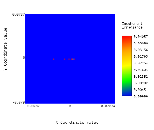
Where n_2(\lambda) is the index of refraction of the material, which is a function of the input wavelength due to the dispersion, and \alpha_{\;top} is the angle at the top of the prism. As shown from this equation, by increasing the angle of the prism, we can increase the resolution. However, we note that we cannot increase the angle too much due to total internal reflection. When the right-hand side of this equation will increase beyond unity, there will be no answer for this equation. In this case, we will have total internal reflection which will prevent the rays from exiting the prism. The size of the prism is important for the resolution since it allows us to resort to larger lenses for better spectral bandwidth and higher resolution. The schematic of the spectrometer is shown in Fig. 3. The resulting measurements of such a spectrometer are shown in Fig. 4.
The other benefits of such spectrometers are the increased spectral bandwidth and the robustness of the system. Therefore, such spectrometers are suitable for analyzing weak signals over a wider bandwidth, where the resolution is less important. It is important to note that such spectrometers are not based on reflection from a grating but on transmission through the prism, and therefore, from an engineering point of view, they are more challenging to fold a large optical scheme into a small box.
Monochromator
Monochromators are devices similar to a spectrometer that is designed to filter a specific spectral component out of an input. Some of them have tunability in the output wavelength and bandwidth, while others are fixed. In these devices, we replace the detector array with a slit, so only a narrow wavelength can pass and send this wavelength as the output. Therefore, monochromators have optical input, which can be broadband and an optical output which is narrowband. By changing the location of the slit the user can tune the output wavelength and by changing the width of the slit the user can set the bandwidth of the output. Since spectrometers and monochromators are similar, many devices have both, meaning, a spectrometer which is also a monochromator, and vice-versa. A schematic of a monochromator that is based on a grating is shown in Fig. 5. It is also possible to design a monochromator-based on prisms. Such monochromator has wider bandwidth but with lower spectral resolution.

Pulse shaper
The monochromator is a basic spectral manipulator that blocks all the spectral components from a single component that is directed as the output. Pulse shapers are more advanced than monochromators, and with them, the user can impose a complex function of both phase and intensity on the spectrum of the input signal. To obtain a pulse shaper, we replace the slit with a spatial light modulator (SLM) that can impose an arbitrary phase or intensity as a function of space.
Pulse shapers have the same resolution and bandwidth considerations as a spectrometer, but now it is impossible to scan the spectral range slowly. Pulse shapers are designed for altering the spectrum of a pulse and thus, shaping the pulse. Therefore, we need to address the entire spectral bandwidth in a single interaction.
Usually, a pulse shaper needs lower resolution but broader spectral bandwidth than spectrometers. Therefore, building the pulse shaper with 4 gratings or prisms instead of two gratings or prisms and two lenses is better. These setups are possible only when the distances between the elements are short since the system does not compensate for diffraction. The benefits of this system are that it is easier to align and it is possible to tune the system bandwidth and resolution only by changing the distances between the elements and without the need to replace the lenses each time. A Schematic of a pulse shaper is shown in Fig. 6, here, we separate the different wavelengths in space and then combine them again into a beam.

Temporal spectrometers
The two main types of spectrometers are grating-based and prism-based spectrometers. Nevertheless, there are other types of spectrometers, each type has different properties and gives different benefits to the system. All types of spectrometers are based on some technique to separate the spectral components so they can be measured separately. Grating and prism-based spectrometers separate the spectral components in space, and measure them with an array of detectors. In this section, we will consider two types of spectrometers that separate the different spectral components in time and not space.
Time stretch
A time stretch-based spectrometer is a spectrometer that is dedicated to measuring the spectrum of pulses or ultrashort input signals. It is based on an element with high dispersion where different spectral components travel at different speeds. Therefore, this system maps the spectrum into time and at the output, we resort to a single fast detector that measures the spectrum of the input signal. The resolution of this system depends on the temporal resolution of the detector and the dispersion of the element, as:
\delta\lambda=\frac D{\delta t}
Where D is the dispersion of the element and δt is the resolution of the detector. In this system, similar to all the other spectrometers, the spectral bandwidth of the spectrometer decreases when the resolution increases. Here the spectral bandwidth is limited by the repetition rate of the incoming signal. If we are measuring a single input pulse, then we can increase it indefinitely in time and obtain as high resolution as we like. However, if the input is a train of pulses, high dispersion will result in adjacent pulses overlapping each other. Therefore, the time between pulses sets the bandwidth according to:
\triangle\lambda=\frac{\triangle t}\beta
Where \triangle t is the timing between input signals, and \beta is the system dispersion.
There are different options for obtaining a large dispersion. The first option is using a long optical fiber. Such optical fibers can have a dispersion of 200 ps/nm/km so resorting to a few km of such fiber gives a high resolution. This technique is suitable for specific wavelengths around the telecom bandwidth. The second option, when working with different wavelengths such as visible, UV, or far IR, is to resort to gratings. Here we design a system where different components travel different optical distances. This is obtained by the system presented in Fig. 7 and is based on two gratings for imposing dispersion on the pulse.

Fabry-Pérot spectrometer
Cavities or resonators are optical components where the light travels several times and interfere with itself in each roundtrip. One of the simplest cavities is the Fabry–Pérot cavity, built from two mirrors directed at each other. If one mirror is a high-reflection mirror and the second one is partially reflecting, the cavity input and output will be from a single side. But, when the cavity is built from two partially reflecting mirrors, the system becomes an effective mirror with a spectral response. This is illustrated in Fig. 8 and the spectral response of the system transparency follows:
t(w)\;=\;\frac1{1-e^{i\beta L}}
Where t is the amplitude transmission, r is the amplitude reflectivity of the mirrors, L is the total length of the cavity, and \beta is the propagation vector of the light. This leads to a perfect transmission for specific wavelengths for βL=π. Therefore, by placing a detector after the cavity and changing the distance between the mirrors, we can measure different spectral components of the input light. This method is idle for cases where the input does not change in time since it takes time to scan the entire spectral bandwidth. The resolution is set by how accurately the motors change the mirror position and the Fiennes of the cavity. By increasing the cavity distance, we can increase the resolution, but then the bandwidth of the system drops. A second problem is that for any distance between the mirrors, any integer wavelength number can satisfy the cavity condition with high transmission and not just a single component. This is considered when designing the system and analyzing the input bandwidth. As long as the input bandwidth is limited, it is possible to design the spectrometer accordingly. If the input bandwidth is wider or equal to an octave, it will be challenging to measure the spectrum with this system.


