Introduction to Optical Lens Properties

VIRTUAL LAB

Introduction to Optical Lens Properties

Course Overview
This laboratory course will introduce the student to the optical properties of lenses through first principles and simulation analysis. Building a foundational knowledge of optical substrates, surface curvature, and best practices for using lenses in optical systems helps bring these concepts together. In this course, a theoretical review of lens optical properties will be followed by simulation exercises with 3DOptix.
Course Duration

Approximately 3 hours (self-paced)

Learning Objectives
By the end of this pre-lab assignment, students should be able to:
  • Understand how optical substrates and surface curvature affect light
  • Calculate the focal length of a lens using the thin and thick lens equations
  • Use the Abbe number to understand the dispersion of a lens
  • Conduct basic analysis on spherical aberration
  • Incorporate best practices for using lenses in an optical system
Course Outline - Introduction to Coherence
Lenses are made of transparent substrates that interact with light by refraction.  The substrate must be able to transmit more light than it absorbs to be useful and hence be called transparent.  For this reason, certain substrates are used over different wavelength ranges.  As an example, lenses made of silica are used from the UV to NIR spectral range while silicon lenses are used in the NIR to LWIR region.  The absorption of light in a substrate is primarily driven by the electronic structure of the material such as band structure, band gaps, and energy levels.  While refraction through an appropriate substrate will change the direction of incident light, curved surfaces must be used to change the behavior of light as it exits it.

Optical Substrates and Surface Curvature

Using a substrate that is transmissive to light and with an appropriate index of refraction the curvature of a lens can be changed to manipulate the light incident upon it.  The radius of curvature can be equated to the focal length of a lens using the lens maker’s equation.  It is assumed the lens is suspended in air (n=1).
1. \frac{1}{f} = (n_l-1){\bigg(}\frac{1}{R_1}-\frac{1}{R_2}+\frac{(n-1)t}{n_lR_1R_2}{\bigg)}
Equation 1 is the lensmaker’s equation and is used for “thick” lenses and assumes both surfaces are curved. This may not always be the case as one surface can be flat or plano.  If one surface is not curved then the lensmaker’s equation can be simplified by taking the radius to be infinity which will make the terms with R2 in the denominator zero.
2. \frac{1}{f} = \frac{n_l-1}{R_1}
This can be further simplified into a “thin” lens equation by setting t in equation 1 to zero.
3. \frac{1}{f} = (n_l-1)\bigg(\frac{1}{R_1}-\frac{1}{R_2}\bigg)
Although the thickness of the lens is not accounted for in this equation a good estimation of focal length can be made.
Fig. 1. A paraxial, bi convex, and a plano-convex lens. These three lenses’ focal lengths can be calculated using equations 1-3.
Experiment 1

Focal Lengths of Various Lenses

Calculating the focal length of a lens is a straightforward process by using equations 1 through 3 from the above section. This can be accomplished by choosing a substrate and varying the radii of curvature for the two surfaces until the desired focal length is achieved. Since the focal length will vary over the wavelength range that it is transparent, it is useful to calculate many values. The next step will be to use the 3DOptix optical design software to verify the information and see the differences in the calculations.
Exercise 1
  • Using Equations 1, 2, and 3 from the previous section fill out the table below.
  • Keep the simulation file open for the next exercise.
Extra information
Designing optical lenses before the computer era involved a meticulous blend of theoretical knowledge and manual calculations. Optical designers relied on established theories of optics, performing intricate mathematical calculations by hand to determine the optimal dimensions and shapes of lenses. The process often included a trial-and-error approach, with designers creating prototypes based on initial calculations and refining designs through experimental setups like optical benches. Iterative adjustments were made until satisfactory performance was achieved. Expertise, experience, and intuition played crucial roles, as designers lacked the computational tools available today. The process was labor-intensive, time-consuming, and heavily reliant on the skills of the designers in understanding and manipulating light.
Exercise 2
  • Go to the menu bar at top and click tools, then select the lens calculator (see fig. 2).
  • Fill out the table below using the values calculated in the lens calculator (see fig. 2).
  • EFL, FFL, and BFL stand for effective, front, and back focal length.
  • Compare the values from focal length calculations in Exercise 1.
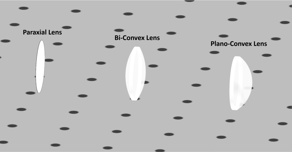
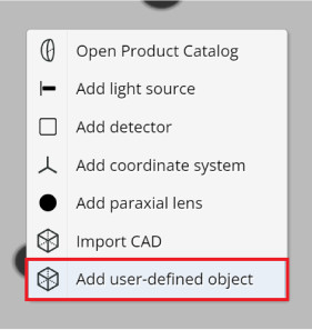
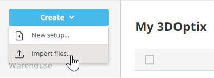
  • Next, in the 3D layout right click and select add user-defined object. 
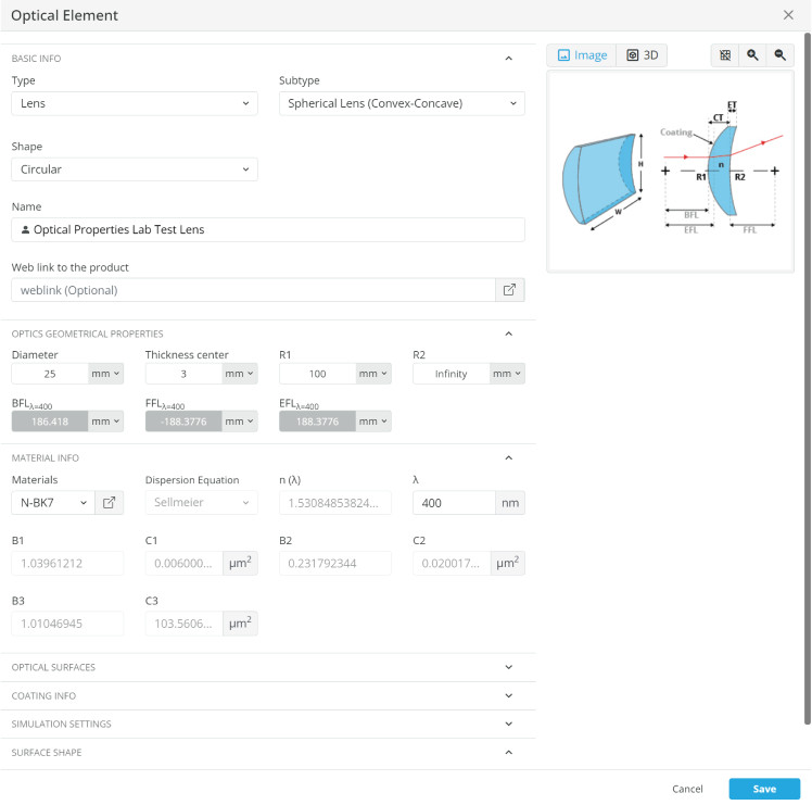
On top of calculating lenses’ values, and adding and modifying lenses from the catalog, a lens can be created using this method.
  • Create lens #1 from Exercise 2 and add to the 3D layout by clicking save.
  • Right click in the 3D layout and select Open Product Catalog.
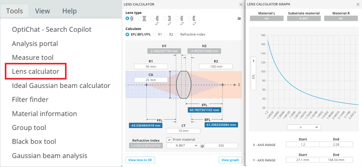
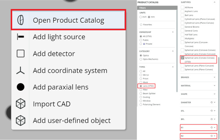
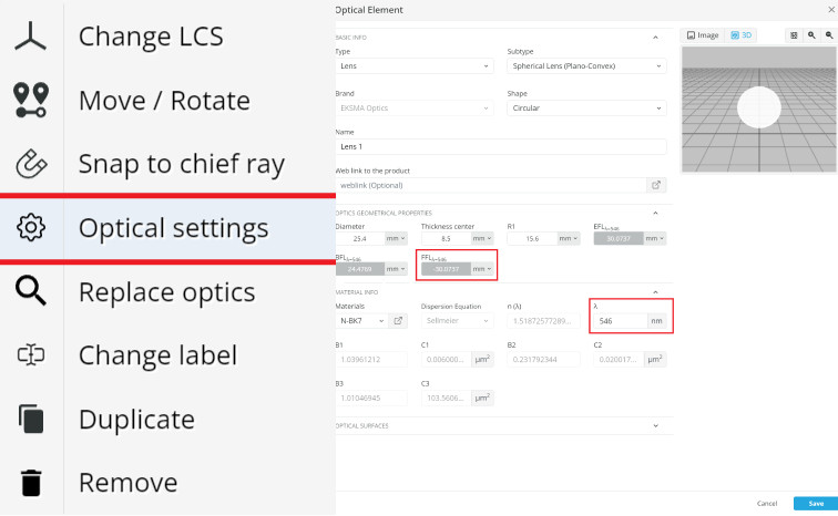
  • Find a lens using the filters on the left that matches the optical properties of the theoretical lens created using the add user-defined object method. This is important for optical designers as ideal theoretical lenses are initially used to create an optical system, then readily available lenses are identified with matching properties for real prototype designs.
Extra information
Optical design with computer software represents a transformative shift from manual methodologies to advanced, efficient, and precise processes. Utilizing specialized software, optical designers can model and simulate complex optical systems with greater accuracy. Computer-aided design (CAD) programs enable the creation and optimization of lens designs through automated calculations, significantly reducing the need for manual computations. This allows for rapid prototyping and virtual testing, facilitating the exploration of various design parameters. Additionally, optimization algorithms enhance the efficiency of the iterative process, enabling designers to quickly converge on optimal solutions. Integration with computational tools streamlines the analysis of aberrations, light paths, and other critical factors.
Experiment 2

Abbe Number and Chromatic Aberration

The Abbe number, also known as the V-number, is a dimensionless number that characterizes the dispersion of a substrate. It is commonly used in optics to describe how much it disperses light into its component colors. The Abbe number is crucial in lens design, particularly in the correction of chromatic aberrations. This value is only used for optical glass transmissive in the visible spectrum as the calculations involved test visible test wavelengths. Generally, the range of values can be placed in the following two groupings.

  • > 55, crown glass, indicates lower dispersion, less sensitivity to chromatic aberrations, more lens curvature needed
  • < 50, flint glass, indicates higher dispersion, more sensitivity to chromatic aberrations, less lens curvature needed

There is an interactive diagram where the abbe number can be found on the Schott website for various optical glasses. Exploring the Abbe number means exploring the wavelength dependency of glass substrates. As the index of refraction changes over the transmissive wavelength range the bending of light rays will not be constant. This affects the manipulation of light and for imaging system the ability to focus light into a small spot.

Fig. 2. A single wavelength collimated light sources enters a lens and focuses down to a very small spot.
Fig. 3. Three collimated light sources at different wavelengths enter a lens and focus at different points. Chromatic aberration is present for all substrate types, but at varying levels depending on the Abbe number. This will create a halo of colors effect when focused.
Exercise 3
  • In the 3DOptix app, import the file “Abbe_FL.opt“.
  • Click on lens 1 and go to the optical settings.
  • Change the wavelength under the material info tab to see the focal lengths for each respective wavelength.
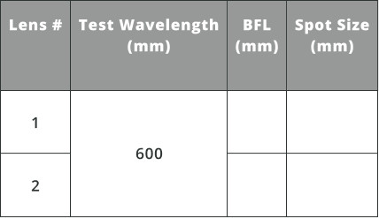
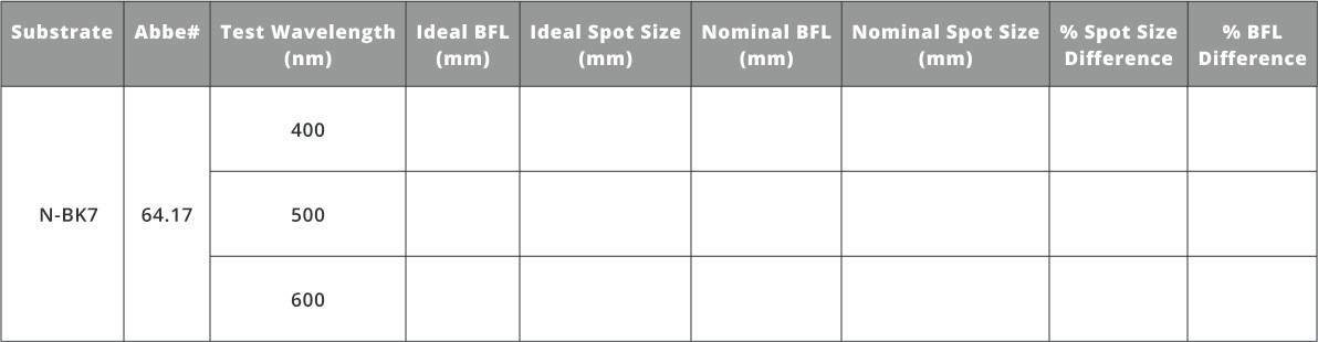
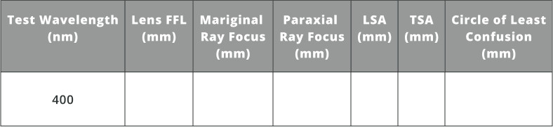
  • Enter the BFL values in the ideal BFL column. 
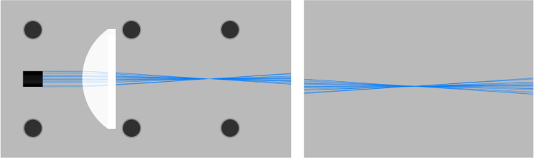
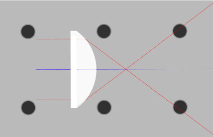
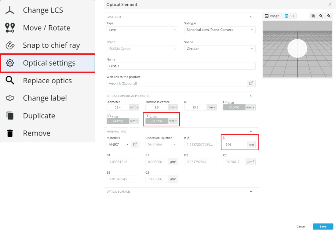
Notice lens 1 front surface (curved) is facing the light source and the Plano surface (back) is facing the detector. Therefore, the BFL is needed for the distance from the detector measurement.
  • Open the analysis window from the menu bar, change the detectors to advanced (Spot Incoherent), 300×300 X/Y pixels, and then run analysis.
  • View the detectors placed at the appropriate foci for the three wavelengths and measure the spot size using the measure mode tool and fit to circle.
  • Enter these values under ideal spot size
  • Now place the three detectors at the ideal BFL of the 500nm test wavelength
  • Enter this value under nominal BFL for each test wavelength
  • Run the analysis again and measure the spot sizes
  • Enter these values under nominal spot size
  • Calculate the difference between the ideal and nominal BFL and spot size for all three test wavelengths
  • The difference in spot size will show up in the final image as chromatic aberration creating rings of different colors
  • Keep the simulation file open for the next exercise
Exercise 4
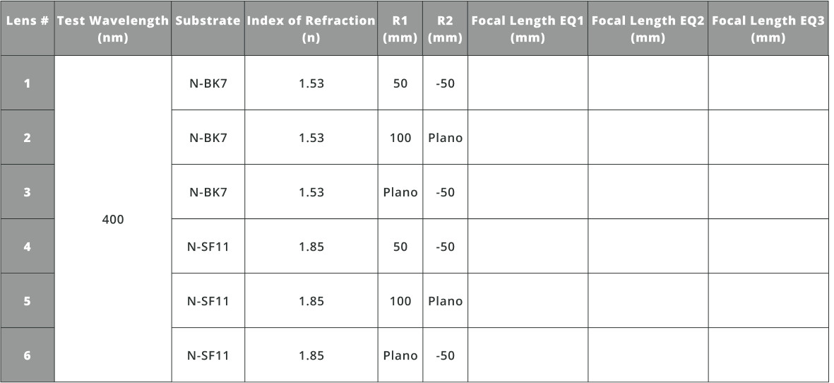
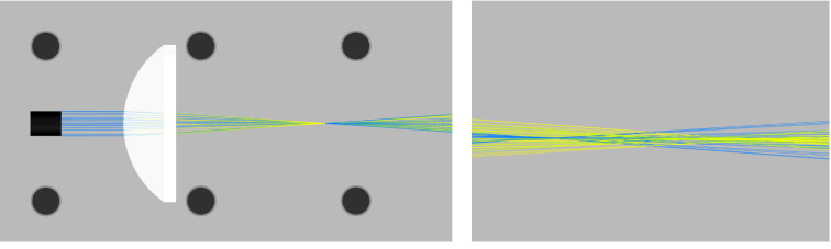
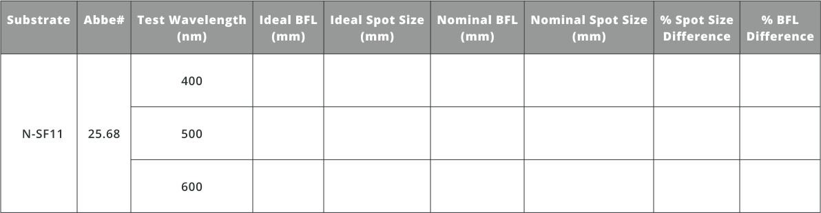
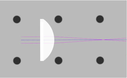
  • This time replace the glass substrate with one having a lower Abbe number; N-SF11. Notice the drastically lower Abbe number, which means higher dispersion.
  • Complete the same analysis completed for N-BK7 lens above.
  • Notice the difference in spot size compared to the N-BK7 lens. This is an important part of chromatic aberration correction.Understanding glass types and their wavelength specific optical properties leads to better designs.
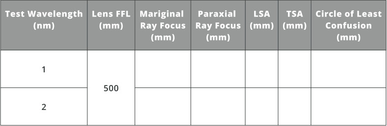
Extra information
In practical terms, the Abbe number is crucial in lens design for optical systems, such as camera lenses, eyeglasses, microscopes, and telescopes. Designers aim to minimize chromatic aberration to improve the overall image quality and clarity. The Abbe number helps in selecting materials for lenses that strike a balance between achieving the desired optical properties and minimizing chromatic aberration.
Experiment 3

Spherical Surfaces and Spherical Aberration

Spherical aberration is an optical phenomenon that occurs when parallel rays of light incident on a spherical lens or mirror do not converge to a single focus. Instead, rays at different distances from the lens optical axis focus at different points. This leads to blurred or distorted images, reducing the optical quality of the system. In optical design, addressing spherical aberration is crucial for achieving high-quality images in devices like cameras, telescopes, microscopes, and eyeglasses. Engineers and lens designers employ various techniques to minimize or correct spherical aberration and optimize the performance of optical systems.
Spherical aberration can be corrected using non-spherical surfaces such as parabolic and aspheric shapes. Analysis is done by tracing rays finding where the marginal and paraxial rays focus lies on the optical axis. There will be both longitudinal (LSA) and transversal (TSA) spherical aberration for any spherical lens. The LSA is measured from the marginal ray focus to the paraxial focus, and the TSA is measured from the paraxial focal plane to where the marginal rays intersect it transversally. The “circle of least confusion” is a plane parallel to the optical axis where the spot size is minimized. This location is given where the smallest spot size can be physically realized.
  • Spherical aberration is proportional to the radial height a ray hits a lens to the fourth power: r4.
Fig. 4. Spherical aberration from a spherical lens. The focus position on the optical axis depends on the ray height at the lens interface.
Fig. 5. The red marginal rays are the rays that intersect the top most point of the lens. These rays attribute the most spherical aberration due to the ray heigth.
Fig. 6. The purple paraxial rays are the rays that intersect nearest the center of the lens and focus nearest the paraxial focus. These rays have very little spherical aberration
To measure the LSA of a lens the distance from the lens surface to the marginal rays focus is measured (fig. 5), then from the lens surface to the paraxial rays focus (fig. 6). The distance between these two foci on the optical axis is the LSA in millimeters.
Fig. 7. Visual representation of LSA
To measure the TSA of a lens the distance to the marginal ray at the paraxial focal plane to the paraxial focus on the optical axis is measured. The distance between these two points is the TSA in millimeters.
Fig. 8. Visual representation of TSA
Finally, the circle of least confusion can be found. This is the location where the distance from the optical axis to highest ray is minimum. In an optical system the imaging component would be placed here.
Fig. 9. Visual representation of the circle of least confusion
Exercise 5
  • In the 3DOptix app, import the file “Spherical_Abb.opt
  • Click on the lens and select optical settings, then change the wavelength to 400nm and record the FFL
  • At the upper right of the screen click the propagation simulation button.
  • There will be seven rays traced through the lens. There is one central ray and six symmetric about the optical axis of the lens simulating rays hitting the same location at the top and bottom. Measure the distance between the lens surface to the two foci in millimeters. See fig. 7.
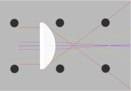
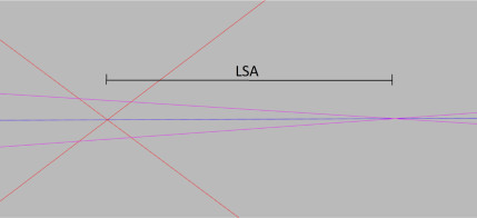
  • Take the foci for each ray pair and subtract these numbers; paraxial focus – marginal ray focus. Positive LSA means the means that marginal rays intersect the optical axis in front of the paraxial focus, and negative if behind it.
  • Measure the TSA by finding the transverse distance to where the marginal ray intersects the paraxial focal plane. See Fig 8.
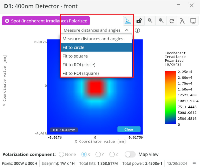
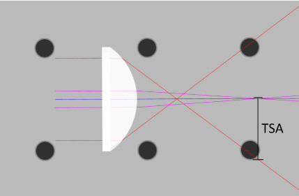
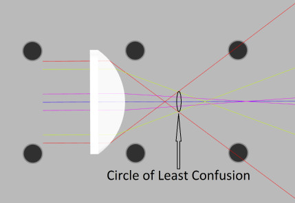
  • Find and measure the circle of least confusion where the marginal rays and paraxial rays meet to create the smallest spot size. See Fig. 9. This is the point where the eye or camera should be placed for best imaging.
  • Record the data in the table below.
Extra information
Originally, optical designers had to manually trace rays through an optical system to determine total spherical aberration present at the image plane. Coupled with various other third-order aberrations this can quickly become difficult to separate. With the advent of computer-assisted design software, this has become exponentially easier as thousands or millions of rays can be traced very quickly and aberrations numerically calculated.
Methods to reduce spherical aberrations are reducing the ray heights when they enter a spherical lens, using non-spherical surfaces, and using equal amounts of positive and negative lenses. These techniques aim to enhance the overall performance of optical systems and achieve better image quality.
Experiment 4

Optical Lenses Best Practices

As a final component of this course an overview of specific best practices and applications will be reviewed. Typically, lens orientations and ray control are pivotal in creating an acceptable optical system that will perform as the optical designer expects. These are “rules of thumb” and “benefits of this method” types of applications that are generally understood through experience in designing and simulating a simple or complex optical system.
Exercise 6
  • In the 3DOptix app, import the file “BP_Spherical.opt“.
  • There are two plano-convex lenses in this file, one with the curved surface facing the light source and one facing the detector. There will be spherical aberration present for both and it is desired to determine the best orientation of the lens to reduce this.
  • Repeat the procedure from Exercise 5 and fill in the table below
Extra information
Notice that spherical aberration is reduced for the configuration of the lens where the curved surface is facing the light source. The reason for this is both surfaces contribute to the spherical aberration since the rays will refract at both interfaces. When the Plano side of the lens faces the light source all the bending of the light happens at the curved surface and the spherical aberration becomes much greater.
Exercise 7
  • In the 3DOptix app, import the file “BP_Collimate-Focus.opt“.
  • There are two lens system configurations in the simulation file similar to Exercise 6. This time it is desired to determine the best orientation for the plano-convex lens to focus to a point.
  • View the detectors placed at the appropriate foci and measure the spot size using the measure mode tool and fit to circle.
Extra information
Notice that spherical aberration is reduced for the configuration of the lens where the curved surface is facing the light source. The reason for this is both surfaces contribute to the spherical aberration since the rays will refract at both interfaces. When the Plano side of the lens faces the light source all the bending of the light happens at the curved surface and the spherical aberration becomes much greater.
Analysis and Conclusion
Optical properties of lenses impact the effectiveness of an optical system and the designer must be aware of the benefits and setbacks to each element and its optical properties. This course has reviewed the fundamental properties of lens substrates, shapes, and basic aberrations. These concepts will become invaluable resources for creating effective optical designs.
Assessment
NA
Resources
The student requires an account in the 3DOptix system.
Synopsys
In this course, students immerse themselves in the captivating realm of light’s interaction with lenses. The curriculum delves into the core principles of light-matter interactions, crucial phenomena that dictate how light behaves at the interface between different optical media. Through engaging experiments and exercises, students acquire a profound comprehension of these concepts and their pragmatic applications.
mascot-1-1

3DOptix works
only on desktop!

Please go to 3doptix.com on a
desktop device, using the
Chrome or Edge browser

Available on January 30th, 2023